Reviewing almost 70 artworks quickly and in depth is a challenge. With _MON3Y AS AN 3RRROR | MON3Y.US, I chose the approach of describing each artwork’s notable features and then pulling out themes and commonalities at the end. Halfway through I realised that by changing each description into a standard format, I could write code to parse the descriptions and analyse them to help me find those themes and commonalities. So I did. The code is in R and it’s available here:
https://github.com/rheaplex/art-review-scripts/
The code loads various modules, parses the file and constructs a corpus and matrix from the words in each review. It then outputs various statistics and graphs regarding them.
First up, which terms do I use most frequently, ten or more times:
 [1] "animated" "bill"     "dollar"   "euro"     "glitched" "image"
 [7] "mapped"   "show"     "texture"  "video"
The most popular subjects are dollar and Euro bills. Art about them shows something about them. It does so using video, animations (whether video, Flash, or HTML5), images, glitch and texture mapping.
Terms I use five or more times:
 [1] "aesthetic"  "animated"   "art"        "background" "banknotes"
 [6] "bill"       "collage"    "colour"     "dollar"     "economic"
[11] "euro"       "flag"       "gif"        "glitched"   "graphic"
[16] "hundred"    "image"      "loop"       "makes"      "mapped"
[21] "money"      "note"       "piece"      "rendering"  "show"
[26] "texture"    "video"      "words"
Flags and words join the subjects, hundred unit notes are the most popular, looped animated GIFs, collages and graphics join the forms and figure/ground relations are there with mention of “background”.
Finally let’s look at words I use three or more times:
 [1] "abstract"    "aesthetic"   "album"       "allow"       "american"
 [6] "animated"    "apparently"  "application" "art"         "background"
[11] "banknotes"   "bill"        "black"       "blue"        "changing"
[16] "classic"     "collage"     "colour"      "composite"   "depicted"
[21] "direct"      "dollar"      "economic"    "effective"   "euro"
[26] "facebook"    "flag"        "flickering"  "frame"       "gif"
[31] "glitched"    "google"      "graphic"     "grid"        "html5"
[36] "hundred"     "image"       "landscape"   "like"        "link"
[41] "loop"        "love"        "makes"       "mapped"      "million"
[46] "money"       "monochrome"  "morphing"    "new"         "note"
[51] "one"         "page"        "patterns"    "piece"       "pixelart"
[56] "playing"     "polygons"    "possibly"    "price"       "rendering"
[61] "screen"      "show"        "signs"       "sites"       "stack"
[66] "style"       "texture"     "time"        "use"         "video"
[71] "virtual"     "web"         "white"       "words"       "work"
[76] "yellow"      "zoomed"
No surprises there, except possibly “love”. The code will confuse “Euro” and “European”, so that’s why the US is mentioned but not Europe. Facebook and Google add corporations to the subjects. Colours are added to the formal properties: yellow, blue, white, black. Landscape joins the subjects. And works play, are direct, are classic, have style, an aesthetic, a price, are new. And I weasel about them with “possibly”.
Next lets look at the associations between words. First some obvious ones.
Money:
google           love          1990s            age        ambient
  0.65           0.59           0.43           0.43           0.43
Art:
corrupted     miscoloured         nothing          purest            rows
     0.75            0.75            0.75            0.75            0.75
   street            look            much           piece         classic
     0.75            0.52            0.52            0.48            0.41
Net:
carefully    contract   described        form        sale    specific
     1.00        1.00        1.00        1.00        1.00        1.00
  another application       price       piece         art
     0.70        0.49        0.44        0.43        0.36
The corruption found in association with art here is aesthetic, thanks to glitch art.
The word cloud in the next section has some stand-out words. We can look at their associations as well to follow suggestions from within the data.
Dollar:
bill                         1950s
0.87                          0.33
Video:
vimeo     amateur      batter       beach     clipart   commodity
 0.40        0.39        0.39        0.39        0.39        0.39
Bill:
dollar                         1950s
  0.87                          0.38
Videos are mostly on Vimeo. Dollar and bill occur together so there’s no surprises there.
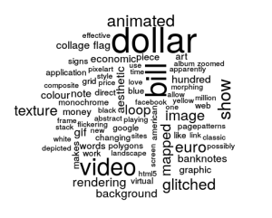
Word clouds are a good way of quickly visualising word frequency. Here’s one of the words in the reviews:
Using the code from my old posts on Vasari’s Lives and on art bloggers we can find the most similar reviews:
Dominik Podsiadly :  JUST DO IT, Jefta Hoekendijk

Maximilian Roganov :  Jasper Elings, Jefta Hoekendijk, Keigo Hara, Alfredo Salazar Caro | TMVRTX, Mathieu St-Pierre

JUST DO IT :  Jefta Hoekendijk, Dominik Podsiadly, Lars Hulst

Mitch Posada :  Dafna Ganani

Lorna Mills & Yoshi Sodeoka :  Jennifer Chan
Jasper Elings :  Maximilian Roganov, Curt Cloninger, Adam Braffman, Δεριζαματζορ Προμπλεμ Ιναυστραλια

Alfredo Salazar Caro | TMVRTX :  Nick Briz, Maximilian Roganov

Dafna Ganani :  Mitch Posada

Jennifer Chan :  Lorna Mills & Yoshi Sodeoka

Jefta Hoekendijk :  JUST DO IT, Maximilian Roganov, Lars Hulst, Dominik Podsiadly

Keigo Hara :  Maximilian Roganov, Nick Briz

Ellectra Radikal :  Lars Hulst

A Bill Miller :  Mathieu St-Pierre

Nicolas Sassoon :  Lars Hulst

Curt Cloninger :  Jasper Elings, Nick Briz
Δεριζαματζορ Προμπλεμ Ιναυστραλια :  Jasper Elings
Lars Hulst :  Ellectra Radikal, JUST DO IT, Jefta Hoekendijk, Nicolas Sassoon

Nick Briz :  Alfredo Salazar Caro | TMVRTX, Keigo Hara, Curt Cloninger

Adam Braffman :  Jasper Elings

Rollin Leonard :  Maximilian Roganov

Mathieu St-Pierre :  A Bill Miller, José Irion Neto, Maximilian Roganov

José Irion Neto :  Mathieu St-Pierre
Do those make sense to look at the art?
The clustering code from the same old posts produces different groupings:
Cluster 1 : Robert B. Lisek, Geraldine Juarez

Cluster 2 : Mitch Posada, Nick Kegeyan, Dafna Ganani, Marco Cadioli, Andrey Keske, Guayayo Coco

Cluster 3 : Rafaël Rozendaal, Adam Ferriss, Aaron Koblin + Takashi Kawashima, Maximilian Roganov, Fabien Zocco, Jasper Elings, Alfredo Salazar Caro | TMVRTX, Anthony Antonellis, Haydi Roket, Keigo Hara, A Bill Miller, Benjamin Berg, Δεριζαματζορ Προμπλεμ Ιναυστραλια, Nick Briz, Vince Mckelvie, Adam Braffman, Rollin Leonard, Mathieu St-Pierre

Cluster 4 : Dominik Podsiadly, Thomas Cheneseau

Cluster 5 : Ciro Múseres

Cluster 6 : Curt Cloninger

Cluster 7 : Miron Tee, Jan Robert Leegte, Paul Hertz, Jon Cates, León David Cobo, Kamilia Kard

Cluster 8 : Nuria Güell, Paolo Cirio, Filipe Matos, Agente Doble | UAFC, JUST DO IT, Gustavo Romano, Tom Galle, Cesar Escudero, Jefta Hoekendijk, Gusti Fink, Ellectra Radikal, Aoto Oouchi, Kim Laughton, Martin Kohout, Marc Stumpel, LaTurbo Avedon, Nicolas Sassoon, Erica Lapadat-Janzen, Milos Rajkovic, Rozita Fogelman, Lars Hulst, Yemima Fink, José Irion Neto

Cluster 9 : Emilio Vavarella

Cluster 10 : Dave Greber, Lorna Mills & Yoshi Sodeoka, Jennifer Chan, Frère Reinert, V5MT, Addie Wagenknecht, Systaime, Émilie Brout & Maxime Marion, Georges Jacotey
I chose ten clusters arbitrarily. There’s some overlap looking at the two techniques.
I wanted to try out Topic Modelling on the data but an algorithm for choosing the optimal number of topics simply returned the same number as there are documents. So I tried 8, 12 and 20.
12 gave “nice” results:
     Topic 1    Topic 2       Topic 3    Topic 4      Topic 5
[1,] "video"    "mapped"      "price"    "bill"       "animated"
[2,] "bill"     "dollar"      "changing" "dollar"     "architectural"
[3,] "dollar"   "texture"     "image"    "love"       "euro"
[4,] "direct"   "bill"        "show"     "artist"     "glitched"
[5,] "facebook" "virtual"     "allow"    "google"     "graphic"
[6,] "faster"   "polygons"    "also"     "money"      "money"
[7,] "page"     "constituent" "analysis" "monochrome" "zoomed"
[8,] "abstract" "exploding"   "another"  "pixelart"   "1990s"
     Topic 6      Topic 7           Topic 8       Topic 9    Topic 10
[1,] "graphic"    "labels"          "dollar"      "dollar"   "texture"
[2,] "abstract"   "landscape"       "glitched"    "euro"     "blank"
[3,] "aesthetic"  "album"           "bill"        "note"     "blue"
[4,] "album"      "animated"        "video"       "animated" "classic"
[5,] "apparently" "appears"         "aesthetic"   "bill"     "economic"
[6,] "banknotes"  "art"             "application" "image"    "essay"
[7,] "european"   "banknotecollage" "colour"      "loop"     "euro"
[8,] "flag"       "banknotes"       "economic"    "american" "show"
     Topic 11     Topic 12
[1,] "bill"       "art"
[2,] "dollar"     "bill"
[3,] "video"      "depicted"
[4,] "background" "dollar"
[5,] "flag"       "labour"
[6,] "loop"       "video"
[7,] "reactive"   "words"
[8,] "roughly"    "1950s"
The topics are clearer with more words, these are just the first few for each one. I think this is the closest to what I want in terms of discovering what I have written about, although as I say the choice is arbitrary (or at least aesthetic rather than statistical).
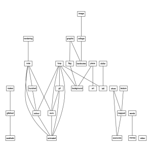
Using more code from the Vasari/bloggers posts, we can plot the associations between words:
Changing the parameters and outputting to PDF creates a more detailed and readable graph. It’s fun and inbetween topic modelling and frequency counts for usefulness.
Finally let’s see how I feel about the art with sentiment analysis:
neutral positive
     66        3
I do try to find the positive in artworks but there was one that gave me an immediate and visceral negative reaction in the show (you can spot it if you look hard at the reviews). I’m surprised that there are fewer that count as positive. I “love” one of the pieces. Is it in the positive list?
[1] "Martin Kohout" "Marc Stumpel" "Ciro Múseres"
It’s not. But one of the ones listed does mention “love”, so I don’t know what’s happened there. Sentiment analysis has improved greatly over the last few years, but apparently not in the library I was using.
If I was going to use these techniques to help review art I’d write longer “bag of word” descriptions for each artwork, with fragments of text and individual words acting almost as tags or streams of consciousness, and I would then use topic modeling and clustering to help pull out themes. I’d prefer to use an algorithm to choose the number of topics, as I feel this is more intellectually defensible, but I like the results enough to use it without. I’m disappointed by the performance of the sentiment analysis library I used, next time I’ll try a different one.
Will there be a next time? Yes, the next time I’m reviewing a group show with more than a few artists. Producing this report has been labour intensive, but I’ve a libary of code now and a better understanding of the issues. And I can automate report construction and revision using Knitr, which would allow me to mix Markdown text and R code without hacing to copy and reformat output.

